Dynsimpie

dynsimpie

A Stata program to examine dynamic compositional dependent variables.

Download

The most recent version of dynsimpie is available on this page. The program can also be found on the SSC RePEc archive, though that link has not been updated in a while.

Table of Contents

• Description
• Requirements
• Syntax
• Required Options
• Additional Options
• Reference
• Authors
• Citations
• Examples
• Example Papers

Description

dynsimpie is a program to dynamically examine compositional dependent variables, detailed in Philips, Rutherford, and Whitten (2016) and used in Philips, Rutherford, and Whitten (2015). Their modeling strategy uses an error correction model within a seemingly unrelated regression to simulate dynamic changes in each compositional dependent variable in response to a counterfactual “shock” to an independent variable during the simulation. Following the work of Aitchison (1986), the program first expresses the dependent variables in compositional form using a log-ratio transformation. dynsimpie then models the first differenced series of each compositional ratio as a function of their lag, as well as the lag and first difference of a vector of independent variables. Expected values are calculated, and, since compositional log ratios are not particularly intuitive, these are then “un-transformed” and the expected (or predicted) average proportion of each dependent variable over time is either graphed and/or saved to a dataset, along with associated confidence intervals.

Requirements

To use dynsimpie, the user must first download and install the Clarify package by King, Tomz, and Wittenberg (2000) (estsimp and setx).

Syntax

dynsimpie indepvars [if] [in] [, options]

• indepvars is a list of independent variables to be included in the model. Independent variables only need to be specified in levels (i.e. un-lagged and un-differenced). The final list of independent variables will be one less than the total number of desired independent variables, since one always has to be specified in the shockvar command (see below). *dynsimpie automatically transforms the dependent variables and independent variables into lags and first differences for estimation in error-correction form. Options on dynsimpie allow for the addition of dummy variables to the model as well as the ability to shock more than one independent variable at the same point in time.

Required options

• dvs(varlist) a list of the compositional dependent variables to be estimated in the model. These must be expressed either as proportions (summing to 1) or as percents (summing to 100). dynsimpie will issue an error message if neither of these criteria are met. dynsimpie will take the log of the proportion of each category relative to the proportion of an arbitrary “baseline” category; for example, if there were J dependent variables in dvs(varlist), dynsimpie would create J-1 categories of s_{tj} = ln(y_{tj}/y_{tJ}), where the Jth category is the baseline. The reason for this is detailed in Philips, Rutherford, and Whitten (2016). Note that J must be 3 or more.
• shockvar(varname) is the independent variable, not included in varlist, that experiences some counterfactual one-period shock at time t. Since this is within an error correction framework, the shock first affects the first difference of shockvar at time t for one period, then will move into the lagged shockvar for the rest of the simulation.
• shock( ) amount to change shockvar(varname) by for one period at time t.

Additional options

• time( ) is the scenario time at which the variable shockvar experiences a one-period shock. By default, this is set at time period 10.
• graph displays a plot of the simulated output. The predicted proportion of each of the compositional dependent variables is plotted against time, along with the associated confidence intervals.
• saving(string) specifies the name of the output file that dynsimpie will save the results to. By default, this is “dynsimpie_results.dta”. This dataset contains a time variable, the midpoints, and upper and lower confidence intervals for each dependent variable. This is commonly used for graphing dynamic simulation results.
• range( ) gives the length of the scenario to simulate. By default, 20 time periods are simulated. range must be greater than the time at which the shock occurs.
• sig( ) specifies the level of confidence associated with the calculation of confidence intervals. If not specified, the default is sig(95) for 95% confidence intervals.
• dummy(varlist) if specified, the program will include these variables as a vector of dummy variables in the model.
• dummyset(numlist) by default, each of the dummy variables in dummy will be set to 0 throughout the simulation. To set them to an alternative value, change the numbers in dummyset. For instance, if specifying dummy(dum1 dum2) and we wanted both dummies set to one, add the option dummyset(1 1).
• shockvar2(varname) allows for an additional shock to take place at time t. As with shockvar, this variable cannot be included in varlist.
• shock2(numlist) is the amount to shock shockvar2( ) by.
• shockvar3(varname) allows for an additional shock to take place at time t. As with shockvar, this variable cannot be included in varlist.
• shock3(numlist) is the amount to shock shockvar3( ) by.
• notable by default, a table of the estimates is shown. This option suppresses the automatic generation of the SUR results.
• nosave by default, dynsimpie will save the results as either “dynsimpie_results.dta” or a user-specified name. This option suppresses this output.
• pv by default, expected values are produced through Clarify. These average out fundamental variability, keeping only estimation uncertainty. Users wishing to analyze both fundamental and estimation uncertainty can do so by generating predicted values with the option pv.

Reference

If you use dynsimpie, please cite us:

Philips, Andrew Q., Amanda Rutherford, and Guy D. Whitten. 2016. “dynsimpie: A command to examine dynamic compositional dependent variables.” Stata Journal 16(3):662-677.

and

Philips, Andrew Q., Amanda Rutherford, and Guy D. Whitten. 2016. “Dynamic pie: A strategy for modeling trade-offs in compositional variables over time.” American Journal of Political Science 60(1): 268-283.

Authors

Andrew Q. Philips, University of Colorado at Boulder, Boulder, CO. andrew.philips [AT] colorado.edu

Amanda Rutherford, Indiana University, Bloomington, IN

Guy D. Whitten, Texas A&M University, College Station, TX

Citations

Aitchison, John. 1986. The statistical analysis of compositional data. Chapman & Hall, Ltd.

Philips, Andrew Q., Amanda Rutherford, and Guy D. Whitten. 2016. “Dynamic pie: A strategy for modeling trade-offs in compositional variables over time.” American Journal of Political Science 60(1): 268-283.

Philips, Andrew Q., Amanda Rutherford, and Guy D. Whitten. 2015. “The dynamic battle for pieces of pie–Modeling party support in multi-party nations.” Electoral Studies 39:264-274.

Tomz, Michael, Jason Wittenberg and Gary King. 2003. “CLARIFY: Software for interpreting and presenting statistical results.” Journal of Statistical Software 8(1):1-30.

Examples

Open the UK data from Philips, Rutherford, & Whitten (2016), which contains data on the proportion of support for the Conservatives (Con), Liberal Democrats (Ldm), and Labour (Lab), during the New Labour government period.

use UK_AJPS.dta, clear

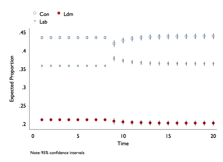
a 1 standard deviation increase of Labour as best manager of the economy at t = 9. By specifying the graph option, dynsimpie automatically produces a time-series plot of the simulations. Note that the results from the seemingly unrelated regression equations are also shown.

dynsimpie all_pidW all_LabLeaderEval_W all_ConLeaderEval_W all_LDLeaderEval_W all_nat_retW, ///
 dvs(Lab Con Ldm) t(9) shock(0.054) shockvar(all_b_mii_lab_pct) graph

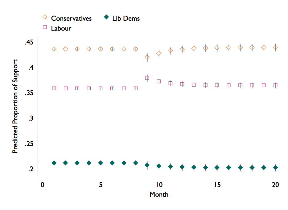
Alternatively, we can open the dataset that dynsimpie produces and graph the results. Note that the program takes the first component in dvs( ) to use as the baseline. When it gets untransformed, this ends up as the LAST predicted category; since we specified dvs(Lab Con Ldm), mid1, mid2, and mid3 correspond with predictions for Con, Ldm, and Lab, respectively.

use dynsimpie_results.dta, clear
twoway rspike var1_pie_ul_ var1_pie_ll_ time || rspike var2_pie_ul_ var2_pie_ll_ time ||   ///
 rspike var3_pie_ul_ var3_pie_ll_ time || scatter mid1 time || scatter mid2 time ||        ///
 scatter mid3 time, legend( order(4 "Conservatives" 5 "Lib Dems" 6 "Labour")) xtitle("Month")     ///
 ytitle("Predicted Proportion of Support")

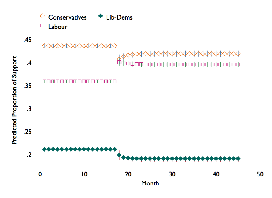
a 1 standard deviation increase of survey respondents who think Labour is the best manager of the economy, along with a 1 standard deviation increase in Labour leader evaluations at time t=18 with range t=45.

dynsimpie all_pidW all_ConLeaderEval_W all_LDLeaderEval_W all_nat_retW ,                  ///
 dvs(Lab Con Ldm) t(18) range(45) shock(0.054) shockvar(all_b_mii_lab_pct)            ///
 shockvar2(all_LabLeaderEval_W) shock2(0.367) nograph
use dynsimpie_results.dta, clear
twoway rspike var1_pie_ul_ var1_pie_ll_ time || rspike var2_pie_ul_ var2_pie_ll_ time ||  ///
 rspike var3_pie_ul_ var3_pie_ll_ time || scatter mid1 time || scatter mid2 time ||       ///
 scatter mid3 time, legend( order(4 "Conservatives" 5 "Lib-Dems" 6 "Labour")) xtitle("Month")    ///
 ytitle("Predicted Proportion of Support")

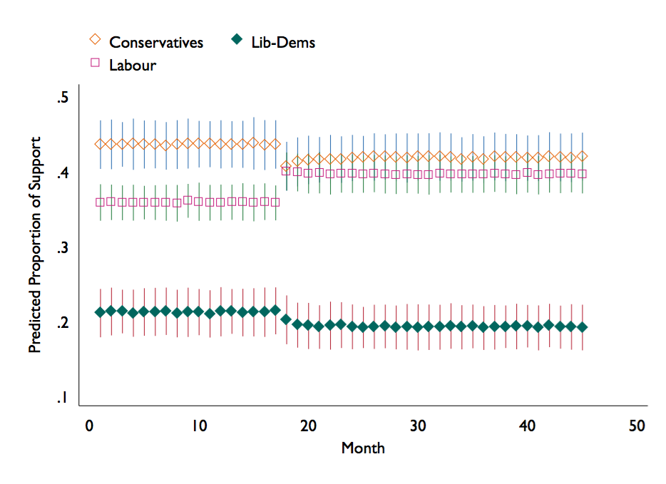
The same as above but generate predicted values instead of expected values.

dynsimpie all_pidW all_ConLeaderEval_W all_LDLeaderEval_W all_nat_retW ,                  ///
 dvs(Lab Con Ldm) t(18) range(45) shock(0.054) shockvar(all_b_mii_lab_pct)            ///
 shockvar2(all_LabLeaderEval_W) shock2(0.367) nograph pv
use dynsimpie_results.dta, clear
twoway rspike var1_pie_ul_ var1_pie_ll_ time || rspike var2_pie_ul_ var2_pie_ll_ time ||  ///
 rspike var3_pie_ul_ var3_pie_ll_ time || scatter mid1 time || scatter mid2 time ||       ///
 scatter mid3 time, legend( order(4 "Conservatives" 5 "Lib-Dems" 6 "Labour")) xtitle("Month")    ///
 ytitle("Predicted Proportion of Support") 

Example Papers

Use dynsimpie in one of your papers? Let me know (aphilips [AT] pols.tamu.edu) and I will add it to the list below: